Melvin Wong managed to defeat the ticking sound issue, good job! https://melvinwong6266.wordpress.com/2016/04/19/day-16-finale-part-2-getting-things-done/

I was going to do this technique myself but I don’t seem to see how it can be done for the way I generate my sequences. (Melvin, if you’re reading this, correct me in the comments if I have made a mistake.)

Melvin appears to generate his sequences using a sort of sliding window approach. So let’s say you have some seed sequence [x1, x2, x3, x4] (this will also be our initial “generated sequence”). You feed this seed sequence to your RNN and get an output [x5]. Now, let’s concatenate [x5] to the generated sequence:

[x1,x2,x3,x4,x5]

Now, let’s remove [x1]:

[x2,x3,x4,x5]

Now, let’s feed [x2,x3,x4,x5] to the RNN and get [x6]:

[x2,x3,x4,x5,x6]

Now, remove [x2]:

[x3,x4,x5,x6]

In this situation, it would make sense that you would get ticking, because you’re feeding [x2,x3,x4,x5] into the RNN and it has no knowledge of [x1]. Likewise, when you feed [x3,x4,x5,x6] into the RNN, it has no knowledge of [x1] or [x2].

I do this technique to generate sequence: given an initial sequence [x1, x2, x3, x4], feed it into the RNN to get [x5]. Now concatenate. Now feed [x1,x2,x3,x4,x5] into the RNN to get [x6]. Now concatenate. Now feed [x1,x2,x3,x4,x5,x6], etc… I always feed the RNN a much longer sequence in each iteration. I can perhaps see this technique as being a perhaps not so good idea, because I train the RNN on fixed length sequences (and at test time it’s getting sequence lengths it’s never seen), but it seems like Melvin’s technique won’t work in my case, because the RNN always gets the “full history” of the generated sequence.

 

GRUV

When I first started on this assignment, one of the first papers I looked at was one called “GRUV: Algorithmic Music Generation using Recurrent Neural Networks”, by two guys at Stanford University. Their task was in comparing GRUs and LSTMs in generating electronic dance music. Here is some EDM they generated on YouTube:

What they do is very similar to what I have done: use LSTMs, and formulate your loss as a regression. But they also convert their raw data into an FFT representation, which was something I tried a while ago but didn’t succeed at (for some reason)! This is what they say:

While audio data is typically represented as samples of a waveform in the time domain, it is usually more meaningful to analyze audio in the frequency domain. After reading the audio samples, we split the audio samples up into blocks of size N and convert each block into its frequency representation using the discrete-Fourier transform (DFT) algorithm. The transformation results in a vector of N real numbers and a vector of N imaginary numbers that collectively make up the phases and magnitudes of the time domain waveform. We concatenate these vectors together to create a 2N vector that is used as the internal model representation for our network.

This sounds exactly what I did! When I looked at the training data that their code produced, it is in the shape (1088, 40, 8000), which means that there are 1088 mini-batches, each mini-batch consisting of 40 sequences, and each of those 40 sequences are 8000-dimensional vectors. This means that , which is 1/4th of a second since the sampling rate is 16,000. This means that each mini-batch is seconds of audio.

The cool thing is that they have some code on Github, and because it’s written in Theano (well, Keras, which is another NN library based on Theano), it was pretty straightforward to set up:

https://github.com/MattVitelli/GRUV

I actually managed to generate some audio with their code, but I only ran the experiment for a short number of epochs, so I don’t want to jump to any hard conclusions yet:

This is an LSTM with 2048 hidden units, trained for ~ 200 epochs. It sounds about the same as the audio I have generated! There is some sense of comfort in this for me.

Interestingly, they say in their code that the number of hidden units should be greater than or equal to the number of frequency dimensions (in our case this is 8000). This is an interesting observation, and short of actually trying to verify this empirically I am not sure I agree because you could easily overfit, no?

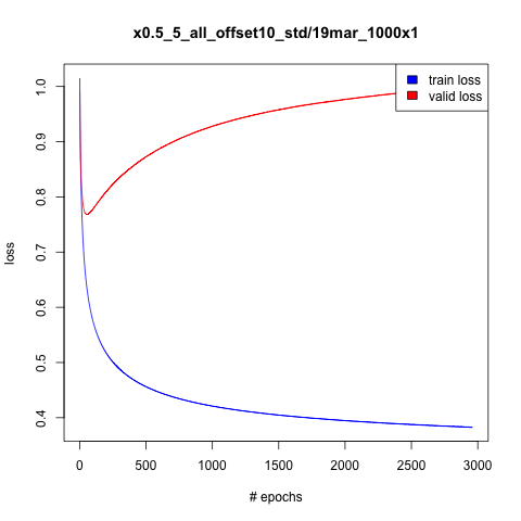
I have been a bit busy lately so I haven’t been doing too much on the assignment. I ran some experiments lately where I simply used my best previous LSTM model and continued training (to save some time) but adding some input layer dropout (). I did get a slight reduction in validation set loss but it isn’t all that much. I also tried adding some gaussian noise to the input and didn’t get anything (). Perhaps it is worth to crank up the dropout probability a bit and see what happens.

I have repeated the previous experiment but this time using 1/10th of a second, e.g. . The audio I generate seems to sound more homogenous, which is not a good thing. This is an interesting result because this experiment uses the same sequence length in seconds as the previous experiment. For example, the previous experiment used of size 2000 (1/8th of a second), with a sequence length of 40, such that 2000*80 / 16000 = 10 seconds, and this experiment we have a sequence length of 100, such that 1600*100 / 16000 = 10 seconds. As of now I am not sure why this is the case.

Here are the learning curves, although I don’t think they’re easily comparable with the previous experiments’ learning curves because we have a different size for , which means we’d expect the squared error to generally be less (imagine the Euclidean distance between two random 2d vectors vs the distance between two random 1000d vectors).

Ok, I’m getting better results now! I ran three experiments last night, each successive experiment adding an extra LSTM layer with 300 units. Here are the learning curves:

We can see that the best model, 300×3 (i.e. 3 hidden layers of 300 units) performs the best in terms of both training and validation loss. Here is some audio I generated with that model using a seed sequence from my test set:

Something I have neglected to mention is that ticking sound, which is something that I have also heard in everyone else’s generated audio. This tick happens between every new chunk of audio that’s generated. For example, for my audio the tick happens very frequently because the length of my input vector is 1/8th of a second (a 2000-dimensional vector). The LSTM doesn’t seem to be good in making a smooth transition between a time chunk and the successive time chunk .

Here is the same experiment as yesterday’s blog but this time using 300 units instead of 600. I have also generated longer audio:

(You get similar sounding audio on seed sequences from the validation and test set.)

I would like to now start looking at having several hidden layers but with a small number of units. Hopefully this makes the LSTM learn a better representation of the audio (therefore also achieving better generalisation on the validation set) and keep the number of parameters reasonable. One of the things that blows up the number of parameters are the connections between the input layer and the hidden layer (since we have 4000 units in the input layer), so if we keep the first hidden layer small then we can add extra hidden layers without blowing up the number of parameters.

Another thing I’d like to experiment with: for this experiment represents a quarter of a second, and we have 40 of these per sequence so that a sequence is seconds long. What if we instead make 1/8th of a second, and keep the sequence length at 10 seconds? I hope that by doing so we will reduce overfitting. By consequence we would also attain a “longer” sequence since it will now be a sequence consisting of 80 elements, since seconds. Having a “longer” memory sounds essential to generate audio that is more diverse.

I decided to run some more experiments and this time use 1) a shorter length (from 0.5 of a second to 0.25 of a second), 2) increase the sequence length to 10 seconds of audio rather than 5, and 3) use fewer hidden units (1000 to 600). The audio I have generated sounds the same as last time but it is good to see that I am overfitting less on the validation set:

It is also nice to see the waveform taking on a more similar shape to the original audio in terms of minimum and maximum amplitude:

In an earlier blog post I mentioned experimenting with transforming the data to the FFt space and training on that. For some reason I wasn’t able to generate anything from that at all (i.e. it was just white noise), but I want to take another crack at it but this time not use min/max normalisation.

I had a look at the blog of fellow student Alex Nguyen and found that he tried different normalisation techniques, one of which was simply dividing the data by its standard deviation. So far I have used min-max normalisation (normalise the data between 0 and 1), but thought maybe scaling the data by the standard deviation is “better”? For starters, the original data takes on both positive and negative values between -8000 to 8000 (approximately), and letting the neural net output negative values might somehow help it during training? He also changed the initial bias value for the forget gate of the LSTM, referring to this comment in the Lasagne docs:

For LSTMLayer the bias of the forget gate is often initialized to a large positive value to encourage the layer initially remember the cell value, see e.g. [R41] page 15.

Because I was short on time, I decided to try both ideas: scale the data by the standard deviation and also initialise my LSTMs with a bias value of 1.0 for the forget gate. I found that (unlike my older experiments) overfitting happened extremely quickly. These are the learning curves for a single-layer LSTM consisting of 1000 units when is an 8000-dimensional vector (i.e. 0.5 of a second).

Fear not! Overfitting is still a good thing and it tells us that our model has sufficient capacity to model the problem. The fact that it overfit really fast tells me that this technique of normalisation converges much faster.

I decided to then generate some audio on the training set using the LSTM:

It doesn’t seem to sound all that different from the last audio I generated, but if you look at the waveform you can see that the amplitudes of the generated audio (~100,000 onwards) nearly matches the amplitudes of the seed sequence, which I think is a really good thing to see.

I am still having trouble generating some audio that sounds good. My latest model produces something that is somewhat interesting but there is still a lot of  “white noise” (note: the nice sound at the start is the seed sequence, wait till the audio gets bad since that is the actual generated audio!):

This is the waveform of the audio:

This is the best model I have generated so far. Looking at my code, I realised that I did some silly things and could have generated *a lot more* training data than I expected. For example,when I was generating sequences by iterating through the training data, I was using a non-overlapping sliding window. Let’s say I have the array [a,b,c,d,e,f,g,h] and my sliding window was a size of 2. I would generate these sequences:

[a,b], [c,d], [e,f], [g,h]

…rather than potentially: [a,b], [b,c], [c,d], …, [f,g], [g,h]

Generating all these sequences however would be really expensive from a memory point of view, but you can still generate more sequences by specifying an “offset” to start from. For example, if my offset was 1, I could generate:

[b,c], [d,e], [f,g]

If the offset is 2, you get: [c,d], [e,f], [g,h] again (which is not what you want), so you should specify offsets that give you different sequences.

Perhaps this is the reason why it has taken me so long to generate good sounding audio — I really needed more training data!

—–

In an earlier blog post I mentioned this paper here:

Click to access NayebiAran.pdf

“While audio data is typically represented as samples of a waveform in the time domain, it is usually more meaningful to analyze audio in the frequency domain. After reading the audio samples, we split the audio samples up into blocks of size N and convert each block into its frequency representation using the discrete-Fourier transform (DFT) algorithm.”

This made me wonder if training in FFT space will make it much easier to generate some decent audio. Also, I found this post on /r/machinelearning:

Training a RNN with audio data
byu/jiminiminimini inMachineLearning

Sander Dieleman says:

“…for now I think using an STFT representation as input is the way to go. It’s just easier to deal with. If you work with raw audio signals your RNN would need an insanely long memory.”

The approach he suggests is similar to what is done in the GRUV paper:

“Complex-valued data isn’t an issue by the way: say you have a complex-valued vector of size 1024 representing an STFT frame, you can convert that into a real-valued vector simply by separating the real and imaginary parts and concatenating them into a vector with 2048 values in total.”

I have just written some prototype code in an IPython notebook to facilitate the conversion of the raw .wav data into an FFT form that is compatible with how Lasagne expects its data.

What’s next

I am currently running some experiments where I’m letting instead, i.e., 1/4 of a second. I feel as if making a 16,000 dimensional vector (i.e. a second of audio) is overfitting, especially when you consider that each value in that vector is assumed to be independent of every other element in the vector.

More to come!